用于眼异常评估的Shack -Hartmann传感器的建模 - 更新的示例#
此示例是知识库础示例的更新版本Modelling of a Shack-Hartmann Sensor for eye aberration evaluation。在特定的情况下,它使用改进的梯度来进行反向的晶体。它使用ZOSPy”`来控制API。
包括功能#
序列模式:
系统设计:
使用
zospy.functions.lde.surface_change_type更改表面类型,包括使用用户定义的表面使用
zospy.functions.lde.surface_change_aperturetype更改特定表面的孔径类型。使用
zospy.solvers.material_model更改表面的材料。使用表面的
PhysicalOpticsData属性来改变特定的物理光学设置使用表面的
coatingData属性来改变特定的涂层设置使用
oss.mce访问多个配置编辑器并指定同一模型的各种配置。使用
oss.SystemData调整特定系统设置
分析:
使用
zospy.analyses.wavefront.zernikestandardceefficients执行Zernike标准系数分析。使用
zospy.analyses.wavefront.wavefrontmap执行波前图分析。使用
zospy.analyses.extendendScene.Demitricimageanalysiss进行几何图像分析。使用
zospy.analyses.physicaloptics.create_beam_parameter_dict以获取和更改特定物理光学传播光束类型的默认光束参数。使用
zospy.analyses.physicaloptics.physicalopticspropagation进行物理光学传播分析。
保修和责任#
提供了示例“原样`。没有保证,也不能从中获得权利,正如该存储库的一般许可中所述。
导入依赖项#
[1]:
from warnings import warn

import matplotlib.pyplot as plt
import pandas as pd

import zospy as zp
from zospy.functions.lde import surface_change_aperturetype, surface_change_type
from zospy.solvers import material_model
初始化OpticStudio#
通过ZOSPy库与Opticstudio建立联系。
在此示例中,我们在扩展模式下与OpticStudio连接。
[ ]:
zos = zp.ZOS()
oss = zos.connect("extension")
直接创建了一个新系统,并确保它处于序列模式。
[ ]:
oss.new()
oss.make_sequential()
True
创建眼睛#
在本节中,我们创建了反向眼模型。请注意,传递给镜头后和镜头前的梯度参数与知识库示例中的参数不同。
为了跟踪我们已经实现的曲面的数量,我们使用了一个叫做n_surf的常量。
[ ]:
n_surf = 0  # Make sure we start at surface 0.

# Object
s_object = oss.LDE.GetSurfaceAt(n_surf)
n_surf += 1
s_object.Thickness = 0

# Retina
s_eye_retina = oss.LDE.InsertNewSurfaceAt(n_surf)
n_surf += 1
s_eye_retina.Comment = "Eye Retina Vitreous"
s_eye_retina.Radius = 12.0
s_eye_retina.Thickness = 17.928551
material_model(s_eye_retina.MaterialCell, refractive_index=1.336, abbe_number=50.23)
s_eye_retina.Conic = 0.0
s_eye_retina.SemiDiameter = 12

# Lens back
s_eye_lens_back = oss.LDE.InsertNewSurfaceAt(n_surf)
n_surf += 1
surface_change_type(s_eye_lens_back, zp.constants.Editors.LDE.SurfaceType.Gradient3)
s_eye_lens_back.Comment = "Eye Lens Back"
s_eye_lens_back.Radius = 8.1
s_eye_lens_back.Thickness = 2.430
s_eye_lens_back.Conic = 0.960
s_eye_lens_back.SemiDiameter = 5
s_eye_lens_back.SurfaceData.DeltaT = 1.0
s_eye_lens_back.SurfaceData.n0 = 1.36799814
s_eye_lens_back.SurfaceData.Nr2 = -1.978e-03
s_eye_lens_back.SurfaceData.Nz1 = 0.03210030
s_eye_lens_back.SurfaceData.Nz2 = -6.605e-03

s_eye_lens_back.PhysicalOpticsData.UseRaysToPropagateToNextSurface = True

# Lens front
s_eye_lens_front = oss.LDE.InsertNewSurfaceAt(n_surf)
n_surf += 1
surface_change_type(s_eye_lens_front, zp.constants.Editors.LDE.SurfaceType.Gradient3)
s_eye_lens_front.Comment = "Eye Lens Front"
s_eye_lens_front.Radius = 0.0
s_eye_lens_front.Thickness = 1.590
s_eye_lens_front.Conic = 0.0
s_eye_lens_front.SemiDiameter = 5
s_eye_lens_front.SurfaceData.DeltaT = 1.0
s_eye_lens_front.SurfaceData.n0 = 1.40699963
s_eye_lens_front.SurfaceData.Nr2 = -1.978e-03
s_eye_lens_front.SurfaceData.Nz1 = 8.6000e-07
s_eye_lens_front.SurfaceData.Nz2 = -0.015427

s_eye_lens_front.PhysicalOpticsData.UseRaysToPropagateToNextSurface = True

# Posterior chamber
s_eye_posterior_chamber = oss.LDE.InsertNewSurfaceAt(n_surf)
n_surf += 1
s_eye_posterior_chamber.Comment = "Posterior chamber"
s_eye_posterior_chamber.Radius = -12.40
s_eye_posterior_chamber.Thickness = 0.0
material_model(s_eye_posterior_chamber.MaterialCell, refractive_index=1.336, abbe_number=50.23)
s_eye_posterior_chamber.Conic = 0.0
s_eye_posterior_chamber.SemiDiameter = 5.0

s_eye_posterior_chamber.PhysicalOpticsData.UseRaysToPropagateToNextSurface = True

# Pupil
s_eye_pupil = oss.LDE.GetSurfaceAt(n_surf)
n_surf += 1
s_eye_pupil.Comment = "Pupil"
s_eye_pupil.Radius = 0.0  # Check
s_eye_pupil.Thickness = 3.160  # Check for oblique rays, if possible remove next surface
material_model(s_eye_pupil.MaterialCell, refractive_index=1.336, abbe_number=50.23)
s_eye_pupil.Conic = 0.0
s_eye_pupil.SemiDiameter = 2.0

surface_change_aperturetype(s_eye_pupil, zp.constants.Editors.LDE.SurfaceApertureTypes.FloatingAperture)

# Cornea back
s_eye_cornea_back = oss.LDE.InsertNewSurfaceAt(n_surf)
n_surf += 1
s_eye_cornea_back.Comment = "Cornea Back"
s_eye_cornea_back.Radius = -6.40
s_eye_cornea_back.Thickness = 0.550
material_model(s_eye_cornea_back.MaterialCell, refractive_index=1.376, abbe_number=50.23)
s_eye_cornea_back.Conic = -0.60
s_eye_cornea_back.SemiDiameter = 5.0

# Cornea front
s_eye_cornea_front = oss.LDE.InsertNewSurfaceAt(n_surf)
n_surf += 1
s_eye_cornea_front.Comment = "Cornea Front"
s_eye_cornea_front.Radius = -7.770
s_eye_cornea_front.Thickness = 0.0
s_eye_cornea_front.Conic = -0.18
s_eye_cornea_front.SemiDiameter = 5.0
MCE#
现在,我们创建了一个反眼睛模型,我们使用多配置编辑器来确保我们可以在同一系统的几个变体之间切换并分析它们。
[ ]:
oss.MCE.ShowEditor()

# Insert extra configurations
oss.MCE.InsertConfiguration(2, False)
oss.MCE.InsertConfiguration(3, False)
True
MCE中的前两个行是IGNM操作数类型,使您可以在特定的配置中忽略某个范围内的表面。尽管这两个行在知识库示例中未使用,但我们将它们保留为一致性。
[ ]:
mce_1 = oss.MCE.GetOperandAt(1)
mce_1.ChangeType(zp.constants.Editors.MCE.MultiConfigOperandType.IGNM)
mce_1.GetOperandCell(1).IntegerValue = 0
mce_1.GetOperandCell(2).IntegerValue = 0
mce_1.GetOperandCell(3).IntegerValue = 0
mce_1.Param1 = s_eye_retina.SurfaceNumber - 1  # minus 1 as param 1 omits object in list
mce_1.Param2 = s_eye_posterior_chamber.SurfaceNumber

mce_2 = oss.MCE.InsertNewOperandAt(2)
mce_2.ChangeType(zp.constants.Editors.MCE.MultiConfigOperandType.IGNM)
mce_2.GetOperandCell(1).IntegerValue = 0
mce_2.GetOperandCell(2).IntegerValue = 0
mce_2.GetOperandCell(3).IntegerValue = 0
# mce_2 gets updated later as it requires the HS sensor
MCE的第三行使用MOFF操作数,可用于注释。它用于描述眼睛模型的三种变体(正常,近视,远视)。
[ ]:
mce_3 = oss.MCE.InsertNewOperandAt(3)
mce_3.ChangeType(zp.constants.Editors.MCE.MultiConfigOperandType.MOFF)
mce_3.GetOperandCell(1).Value = "Normal"
mce_3.GetOperandCell(2).Value = "Myopia"
mce_3.GetOperandCell(3).Value = "Hyperopia"
MCE的第四行使用THIC操作数,可用于改变特定表面的厚度。它用于在眼模模型的三个状态(正常,近视,远视)之间变化玻璃体的长度。
[ ]:
mce_4 = oss.MCE.InsertNewOperandAt(4)
mce_4.ChangeType(zp.constants.Editors.MCE.MultiConfigOperandType.THIC)
mce_4.Param1 = s_eye_retina.SurfaceNumber
mce_4.GetOperandCell(1).DoubleValue = 17.928551048789998
mce_4.GetOperandCell(2).DoubleValue = 25.000  # 27.000
mce_4.GetOperandCell(3).DoubleValue = 11.000  # 13.000
系统设置#
现在,我们调整一些系统设置,以确保我们具有与知识库示例相同的设置。
[ ]:
# Aperture
oss.SystemData.Aperture.ApertureType = zp.constants.SystemData.ZemaxApertureType = (
    zp.constants.SystemData.ZemaxApertureType.FloatByStopSize
)
oss.SystemData.Aperture.ApodizationType = zp.constants.SystemData.ZemaxApodizationType.Gaussian
oss.SystemData.Aperture.ApodizationFactor = 1.0

oss.SystemData.Aperture.AFocalImageSpace = False  # True <- file of example does not have afocal image space

# Rayaiming
oss.SystemData.RayAiming.RayAiming = zp.constants.SystemData.RayAimingMethod.Paraxial

# Advanced
oss.SystemData.Advanced.ReferenceOPD = zp.constants.SystemData.ReferenceOPDSetting.Absolute
oss.SystemData.Advanced.HuygensIntegralMethod = zp.constants.SystemData.HuygensIntegralSettings.Planar

# Wavelength
wl1 = oss.SystemData.Wavelengths.GetWavelength(1)
wl1.Wavelength = 0.830
望远镜#
在本节中,我们定义了眼睛和Shack-Hartmann传感器之间的两个望远镜。
望远镜1#
望远镜1由6个表面组成,有些表面孔或涂层不同。
[ ]:
# Telescope 1 - surface 1
s_tel1_1 = oss.LDE.InsertNewSurfaceAt(n_surf)
n_surf += 1
s_tel1_1.Radius = 0.0
s_tel1_1.Thickness = 95.200
s_tel1_1.SemiDiameter = 10

# Telescope 1 - surface 2
s_tel1_2 = oss.LDE.InsertNewSurfaceAt(n_surf)
n_surf += 1
s_tel1_2.Radius = 102.5
s_tel1_2.Thickness = 5.0
s_tel1_2.Material = "N-BK7"
s_tel1_2.SemiDiameter = 14.5
s_tel1_2.ChipZone = 0.5

surface_change_aperturetype(
    s_tel1_2,
    zp.constants.Editors.LDE.SurfaceApertureTypes.CircularAperture,
    maximum_radius=14.5,
)

s_tel1_2.CoatingData.Coating = "THORB"

# Telescope 1 - surface 3
s_tel1_3 = oss.LDE.InsertNewSurfaceAt(n_surf)
n_surf += 1
s_tel1_3.Radius = -102.5
s_tel1_3.Thickness = 199.0
s_tel1_3.SemiDiameter = 14.5
s_tel1_3.ChipZone = 0.5

s_tel1_3.CoatingData.Coating = "THORB"

# Telescope 1 - surface 4
s_tel1_4 = oss.LDE.InsertNewSurfaceAt(n_surf)
n_surf += 1
s_tel1_4.Radius = 102.5
s_tel1_4.Thickness = 5.0
s_tel1_4.Material = "N-BK7"
s_tel1_4.SemiDiameter = 14.5
s_tel1_4.ChipZone = 0.5

surface_change_aperturetype(
    s_tel1_4,
    zp.constants.Editors.LDE.SurfaceApertureTypes.CircularAperture,
    maximum_radius=14.5,
)

s_tel1_4.CoatingData.Coating = "THORB"

# Telescope 1 - surface 5
s_tel1_5 = oss.LDE.InsertNewSurfaceAt(n_surf)
n_surf += 1
s_tel1_5.Radius = -102.5
s_tel1_5.Thickness = 99.5
s_tel1_5.SemiDiameter = 14.5
s_tel1_5.ChipZone = 0.5

s_tel1_5.CoatingData.Coating = "THORB"

# Telescope 1 - surface 6
s_tel1_6 = oss.LDE.InsertNewSurfaceAt(n_surf)
n_surf += 1
s_tel1_6.Comment = "ph"
s_tel1_6.Radius = 0.0
s_tel1_6.Thickness = 0.0
s_tel1_6.SemiDiameter = 6.0

surface_change_aperturetype(
    s_tel1_6,
    zp.constants.Editors.LDE.SurfaceApertureTypes.CircularObscuration,
    minimum_radius=6,
    maximum_radius=12,
)
我们还将望远镜1的表面6作为全局坐标参考。
[ ]:
s_tel1_6.TypeData.IsGlobalCoordinateReference = True
望远镜2#
望远镜2由9个表面组成,有些表面孔径类型或涂层不同。
[ ]:
# Telescope 2 - surface 1
s_tel2_1 = oss.LDE.InsertNewSurfaceAt(n_surf)
n_surf += 1
s_tel2_1.Radius = 0.0
s_tel2_1.Thickness = 99.5
s_tel2_1.SemiDiameter = 6.0
s_tel2_1.MechanicalSemiDiameter = 12.0

# Telescope 2 - surface 2
s_tel2_2 = oss.LDE.InsertNewSurfaceAt(n_surf)
n_surf += 1
s_tel2_2.Radius = 102.5
s_tel2_2.Thickness = 5.0
s_tel2_2.Material = "N-BK7"
s_tel2_2.SemiDiameter = 14.5
s_tel2_2.ChipZone = 0.5

surface_change_aperturetype(
    s_tel2_2,
    zp.constants.Editors.LDE.SurfaceApertureTypes.CircularAperture,
    maximum_radius=14.5,
)

s_tel2_2.CoatingData.Coating = "THORB"

# Telescope 2 - surface 3
s_tel2_3 = oss.LDE.InsertNewSurfaceAt(n_surf)
n_surf += 1
s_tel2_3.Radius = -102.5
s_tel2_3.Thickness = 99.5
s_tel2_3.SemiDiameter = 14.5
s_tel2_3.ChipZone = 0.5

s_tel2_3.CoatingData.Coating = "THORB"

# Telescope 2 - surface 4
s_tel2_4 = oss.LDE.InsertNewSurfaceAt(n_surf)
n_surf += 1
s_tel2_4.Comment = "ph"
s_tel2_4.Radius = 0.0
s_tel2_4.Thickness = 0.0
s_tel2_4.SemiDiameter = 3.0

surface_change_aperturetype(
    s_tel2_4,
    zp.constants.Editors.LDE.SurfaceApertureTypes.CircularObscuration,
    minimum_radius=20,
    maximum_radius=20,
)

# Telescope 2 - surface 5
s_tel2_5 = oss.LDE.InsertNewSurfaceAt(n_surf)
n_surf += 1
s_tel2_5.Radius = 0.0
s_tel2_5.Thickness = 99.5
s_tel2_5.SemiDiameter = 14.5

# Telescope 2 - surface 6
s_tel2_6 = oss.LDE.InsertNewSurfaceAt(n_surf)
n_surf += 1
s_tel2_6.Radius = 102.5
s_tel2_6.Thickness = 5.0
s_tel2_6.Material = "N-BK7"
s_tel2_6.SemiDiameter = 14.5
s_tel2_6.ChipZone = 0.5

surface_change_aperturetype(
    s_tel2_6,
    zp.constants.Editors.LDE.SurfaceApertureTypes.CircularAperture,
    maximum_radius=14.5,
)

s_tel2_6.CoatingData.Coating = "THORB"

# Telescope 2 - surface 7
s_tel2_7 = oss.LDE.InsertNewSurfaceAt(n_surf)
n_surf += 1
s_tel2_7.Radius = -102.5
s_tel2_7.Thickness = 0.0
s_tel2_7.SemiDiameter = 14.5
s_tel2_7.ChipZone = 0.5

s_tel2_7.CoatingData.Coating = "THORB"

# Telescope 2 - surface 8
s_tel2_8 = oss.LDE.InsertNewSurfaceAt(n_surf)
n_surf += 1
s_tel2_8.Radius = 0.0
s_tel2_8.Thickness = 99.5
s_tel2_8.SemiDiameter = 6

# Telescope 2 - surface 9
s_tel2_9 = oss.LDE.InsertNewSurfaceAt(n_surf)
n_surf += 1
s_tel2_9.Radius = 0.0
s_tel2_9.Thickness = 0.0
Shack-Hartmann传感器#
现在,我们创建了Shack-Hartmann传感器。它由三个表面组成。请注意,在Surface 1上,我们确保ResampleAfterRefraction打开并配置。我们还使用用户定义的表面,并具有表面2的特定设置。
[ ]:
# Shack-Hartmann sensor - surface 1
s_hs_1 = oss.LDE.InsertNewSurfaceAt(n_surf)
n_surf += 1
s_hs_1.Radius = 0.0
s_hs_1.Thickness = 1.200
s_hs_1.Material = "LITHOSIL-Q"
s_hs_1.SemiDiameter = 6.000

s_hs_1.PhysicalOpticsData.ResampleAfterRefraction = True
s_hs_1.PhysicalOpticsData.XSampling = zp.constants.Editors.LDE.XYSampling.S1024
s_hs_1.PhysicalOpticsData.YSampling = zp.constants.Editors.LDE.XYSampling.S1024
s_hs_1.PhysicalOpticsData.XWidth = 10
s_hs_1.PhysicalOpticsData.YWidth = 10

surface_change_aperturetype(
    s_hs_1,
    zp.constants.Editors.LDE.SurfaceApertureTypes.RectangularAperture,
    x_half_width=6,
    y_half_width=6,
)

# Shack-Hartmann sensor - surface 2
s_hs_2 = oss.LDE.InsertNewSurfaceAt(n_surf)
n_surf += 1
surface_change_type(s_hs_2, zp.constants.Editors.LDE.SurfaceType.UserDefined, filename="us_array.dll")
s_hs_2.Radius = -2.00
s_hs_2.Thickness = 5.600
s_hs_2.SemiDiameter = 6.000
s_hs_2.GetSurfaceCell(zp.constants.Editors.LDE.SurfaceColumn.Par1).DoubleValue = 35.000
s_hs_2.GetSurfaceCell(zp.constants.Editors.LDE.SurfaceColumn.Par2).DoubleValue = 35.000
s_hs_2.GetSurfaceCell(zp.constants.Editors.LDE.SurfaceColumn.Par3).DoubleValue = 0.150
s_hs_2.GetSurfaceCell(zp.constants.Editors.LDE.SurfaceColumn.Par4).DoubleValue = 0.150

s_hs_2.PhysicalOpticsData.OutputPilotRadius = zp.constants.Editors.LDE.PilotRadiusMode.Plane

apd = s_hs_2.ApertureData.CreateApertureTypeSettings(zp.constants.Editors.LDE.SurfaceApertureTypes.RectangularAperture)
apd.XHalfWidth = 6
apd.YHalfWidth = 6
s_hs_2.ApertureData.ChangeApertureTypeSettings(apd)

# Shack-Hartmann sensor - surface 3
s_hs_3 = oss.LDE.GetSurfaceAt(n_surf)
n_surf += 1
s_hs_3.Radius = 0.0
s_hs_3.SemiDiameter = 14.5
s_hs_3.MechanicalSemiDiameter = 14.5
不要忘记更新MCE操作数2(MCE_2),因为这需要定义Shack-Hartmann传感器。
[ ]:
mce_2.Param1 = s_hs_1.SurfaceNumber - 1  # minus 1 as param 1 omits object in list
mce_2.Param2 = s_hs_2.SurfaceNumber
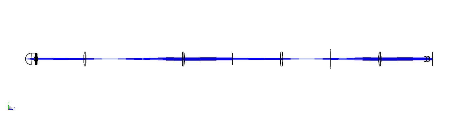
可视化系统#
[ ]:
draw3d = zp.analyses.systemviewers.Viewer3D(
    number_of_rays=7,
    hide_x_bars=True,
    surface_line_thickness="Thick",
    rays_line_thickness="Thick",
    image_size=(2400, 600),
).run(oss)

if zos.version < (24, 1, 0):
    warn("Exporting the 3D viewer data is not available for this version of OpticStudio.")
else:
    plt.figure(figsize=(20, 10))
    plt.imshow(draw3d.data)
    plt.axis("off")
分析#
现在,我们使用各种方法分析系统。
Zernike标准系数#
首先,我们使用“ zp.analyses.wavefront.ZernikestandardCoefficents”评估系统的畸变。
[ ]:
zern = zp.analyses.wavefront.ZernikeStandardCoefficients(
    sampling="64x64",
    maximum_term=37,
    wavelength=1,
    field=1,
    reference_opd_to_vertex=False,
    surface=22,
).run(oss)
[ ]:
pd.DataFrame(zern.data.coefficients.values(), index=zern.data.coefficients.keys())
| value | formula | |
|---|---|---|
| 1 | -8.058524e-01 | 1 |
| 2 | 0.000000e+00 | 4^(1/2) (p) * COS (A) |
| 3 | 0.000000e+00 | 4^(1/2) (p) * SIN (A) |
| 4 | -7.042877e-01 | 3^(1/2) (2p^2 - 1) |
| 5 | 0.000000e+00 | 6^(1/2) (p^2) * SIN (2A) |
| 6 | 0.000000e+00 | 6^(1/2) (p^2) * COS (2A) |
| 7 | 0.000000e+00 | 8^(1/2) (3p^3 - 2p) * SIN (A) |
| 8 | 0.000000e+00 | 8^(1/2) (3p^3 - 2p) * COS (A) |
| 9 | 0.000000e+00 | 8^(1/2) (p^3) * SIN (3A) |
| 10 | 0.000000e+00 | 8^(1/2) (p^3) * COS (3A) |
| 11 | -1.884556e-01 | 5^(1/2) (6p^4 - 6p^2 + 1) |
| 12 | 0.000000e+00 | 10^(1/2) (4p^4 - 3p^2) * COS (2A) |
| 13 | 0.000000e+00 | 10^(1/2) (4p^4 - 3p^2) * SIN (2A) |
| 14 | -1.000000e-08 | 10^(1/2) (p^4) * COS (4A) |
| 15 | 0.000000e+00 | 10^(1/2) (p^4) * SIN (4A) |
| 16 | 0.000000e+00 | 12^(1/2) (10p^5 - 12p^3 + 3p) * COS (A) |
| 17 | 0.000000e+00 | 12^(1/2) (10p^5 - 12p^3 + 3p) * SIN (A) |
| 18 | 0.000000e+00 | 12^(1/2) (5p^5 - 4p^3) * COS (3A) |
| 19 | 0.000000e+00 | 12^(1/2) (5p^5 - 4p^3) * SIN (3A) |
| 20 | 0.000000e+00 | 12^(1/2) (p^5) * COS (5A) |
| 21 | 0.000000e+00 | 12^(1/2) (p^5) * SIN (5A) |
| 22 | -2.780240e-03 | 7^(1/2) (20p^6 - 30p^4 + 12p^2 - 1) |
| 23 | 0.000000e+00 | 14^(1/2) (15p^6 - 20p^4 + 6p^2) * SIN (2A) |
| 24 | 0.000000e+00 | 14^(1/2) (15p^6 - 20p^4 + 6p^2) * COS (2A) |
| 25 | 0.000000e+00 | 14^(1/2) (6p^6 - 5p^4) * SIN (4A) |
| 26 | 1.100000e-07 | 14^(1/2) (6p^6 - 5p^4) * COS (4A) |
| 27 | 0.000000e+00 | 14^(1/2) (p^6) * SIN (6A) |
| 28 | 0.000000e+00 | 14^(1/2) (p^6) * COS (6A) |
| 29 | 0.000000e+00 | 16^(1/2) (35p^7 - 60p^5 + 30p^3 - 4p) * SIN (A) |
| 30 | 0.000000e+00 | 16^(1/2) (35p^7 - 60p^5 + 30p^3 - 4p) * COS (A) |
| 31 | 0.000000e+00 | 16^(1/2) (21p^7 - 30p^5 + 10p^3) * SIN (3A) |
| 32 | 0.000000e+00 | 16^(1/2) (21p^7 - 30p^5 + 10p^3) * COS (3A) |
| 33 | 0.000000e+00 | 16^(1/2) (7p^7 - 6p^5) * SIN (5A) |
| 34 | 0.000000e+00 | 16^(1/2) (7p^7 - 6p^5) * COS (5A) |
| 35 | 0.000000e+00 | 16^(1/2) (p^7) * SIN (7A) |
| 36 | 0.000000e+00 | 16^(1/2) (p^7) * COS (7A) |
| 37 | -4.970000e-06 | 9^(1/2) (70p^8 - 140p^6 + 90p^4 - 20p^2 + 1) |
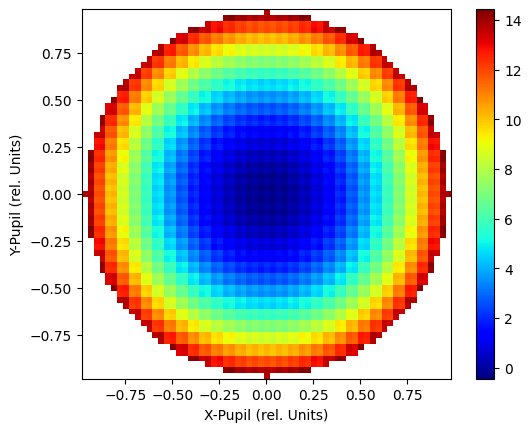
波前图#
我们使用“ ZP.Analyses.wavefront.wavefrontmap`创建波前地图。
[ ]:
wm = zp.analyses.wavefront.WavefrontMap(
    sampling="64x64",
    wavelength=1,
    field=1,
    surface="Image",
    show_as="Surface",
    rotation="Rotate_0",
    scale=1,
    polarization=None,
    reference_to_primary=False,
    remove_tilt=False,
    use_exit_pupil=True,
).run(oss, oncomplete="Release")
[ ]:
fig, ax = plt.subplots()
cbar = ax.imshow(
    wm.data,
    cmap="jet",
    extent=[
        wm.data.columns.values[0],
        wm.data.columns.values[-1],
        wm.data.index.values[0],
        wm.data.index.values[-1],
    ],
    origin="lower",
)

ax.set_xlabel("X-Pupil (rel. Units)")
ax.set_ylabel("Y-Pupil (rel. Units)")
_ = fig.colorbar(cbar)
几何图像分析#
我们还使用zp.analyses.extendendendscene.GeometricImageAnalysis进行几何图像分析。
[ ]:
gia = zp.analyses.extendedscene.GeometricImageAnalysis(
    field_size=0,
    image_size=5,
    wavelength=1,
    field=1,
    file="CIRCLE.IMA",
    rotation=0,
    rays_x_1000=500,
    surface=25,
    show_as="CrossX",
    row_column_number="Center",
    source="Uniform",
    number_of_pixels=300,
    use_polarization=True,
    total_watts=1,
    remove_vignetting_factors=False,
    scatter_rays=False,
    parity="Even",
    delete_vignetted=False,
    use_pixel_interpolation=False,
    reference="Vertex",
).run(oss, oncomplete="Release")
[ ]:
fig, ax = plt.subplots()
cbar = ax.imshow(
    gia.data,
    cmap="gray_r",
    extent=[
        gia.data.columns.values[0],
        gia.data.columns.values[-1],
        gia.data.index.values[0],
        gia.data.index.values[-1],
    ],
    origin="lower",
)

ax.axes.get_xaxis().set_ticks([])
ax.axes.get_yaxis().set_ticks([])

_ = fig.colorbar(cbar)
[ ]:
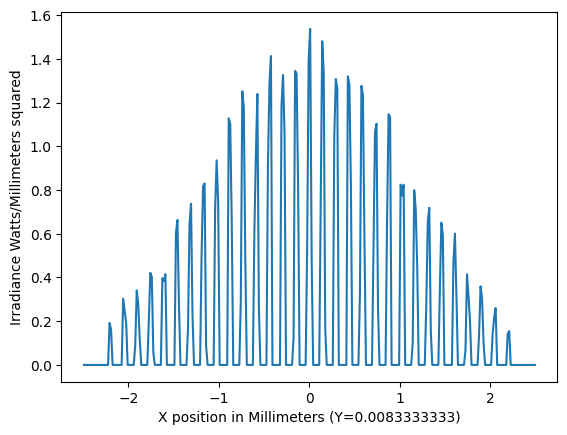
fig, ax = plt.subplots()
data = gia.data.iloc[150]
cbar = ax.plot(
    data,
)
ax.set_xlabel(f"X position in Millimeters (Y={gia.data.index[150]})")
ax.set_ylabel("Irradiance Watts/Millimeters squared")
Text(0, 0.5, 'Irradiance Watts/Millimeters squared')
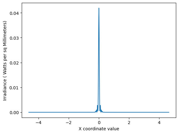
物理光学传播#
最后,我们使用zp.analyses.physicaloptics.physicalopticspropagation进行物理光学传播分析。
注意,我们首先使用ZOSpy辅助函数zp.analyses.physicaloptics.create_beam_parameter_dict来创建一个字典,该字典可以作为光束参数传递给zp.analyses.physicaloptics.PhysicalOpticsPropagation
[ ]:
beam_params = pop = zp.analyses.physicaloptics.create_beam_parameter_dict(oss, beam_type="TopHat")
[ ]:
beam_params
{'Waist X': 2.0, 'Waist Y': 2.0, 'Decenter X': 0.0, 'Decenter Y': 0.0}
[ ]:
beam_params["Waist X"] = 5.4
beam_params["Waist X"] = 5.4
beam_params["Decenter X"] = 0.0
beam_params["Decenter Y"] = 0.0
[ ]:
pop = zp.analyses.physicaloptics.PhysicalOpticsPropagation(
    start_surface=1,
    end_surface="Image",
    wavelength=1,
    field=1,
    surface_to_beam=0,
    use_polarization=False,
    separate_xy=False,
    beam_type="TopHat",
    x_sampling=512,
    y_sampling=512,
    x_width=0.112,
    y_width=0.112,
    use_total_power=True,
    use_peak_irradiance=False,
    total_power=1,
    beam_parameters=beam_params,
    show_as="CrossX",
    data_type="Irradiance",
    project="AlongBeam",
    row_or_column="Center",
    scale_type="Linear",
    zoom_in="NoZoom",
    zero_phase_level=0.001,
    compute_fiber_coupling_integral=False,
).run(oss, oncomplete="Release")
[ ]:
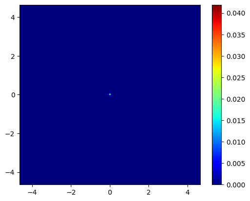
fig, ax = plt.subplots()
cbar = ax.imshow(
    pop.data,
    cmap="jet",
    extent=[
        pop.data.columns.values[0],
        pop.data.columns.values[-1],
        pop.data.index.values[0],
        pop.data.index.values[-1],
    ],
    origin="lower",
)

_ = fig.colorbar(cbar)
[ ]:
fig, ax = plt.subplots()
data = pop.data.iloc[512]
cbar = ax.plot(
    data,
)
ax.set_xlabel("X coordinate value")
ax.set_ylabel("Irradiance ( Watts per sq Millimeters)")
Text(0, 0.5, 'Irradiance ( Watts per sq Millimeters)')