This page was generated from a Jupyter notebook.
Check the source code
or download the notebook..
在双高斯镜头上的射线缩放分析#
此示例显示了如何在双高斯镜头中确定,执行和随后绘制单根光线追迹和光线扇分析。代码取决于由OpticStudio提供的示例文件“ Double Gauss 28 degree field” 。可视化是由Seaborn创建的。
包括功能#
序列模式:
使用“ zospy.analyses.raysandspots.singleraytrace”执行单根光线追迹。
使用“ zospy.Analysis.Raysandspots.Rayfan”执行光线扇分析。
保修和责任#
提供了示例“原样”。没有保证,也不能从中获得权利,正如该存储库的一般许可中所述。
##导入依赖项
[1]:
from pathlib import Path

import matplotlib.pyplot as plt
import numpy as np
import seaborn as sns

import zospy as zp
输入变量
[2]:
# Number of rays per field
number_of_rays = 3

# Field coordinates, as angles w.r.t. the entrance pupil
fields = [0, 10 / 14, 1]

# Plot colors for fields and wavelengths
colors = ["b", "g", "r"]
在独立模式下连接到Opticstudio。独立模式下的分析要比扩展模式下的速度要快得多,因为无需更新用户界面。
[3]:
zos = zp.ZOS()
oss = zos.connect(mode="standalone")
加载Double Gauss 28 degree field。
[4]:
system_file = Path(zos.Application.SamplesDir) / "Sequential/Objectives/Double Gauss 28 degree field.zmx"
oss.load(system_file)
单根光线分析#
为每个视场执行单根光线分析并绘制结果。
[ ]:
# Loop through field coordinates
for i, hy in enumerate(fields):
    # Loop through pupil coordinates
    for py in np.linspace(-1, 1, number_of_rays):
        # Run single ray trace
        raytrace_result = zp.analyses.raysandspots.SingleRayTrace(
            hy=hy, py=py, wavelength=2, global_coordinates=True, field=0
        ).run(oss)

        # Extract real ray data
        rays = raytrace_result.data.real_ray_trace_data

        sns.lineplot(
            rays,
            x="Z-coordinate",
            y="Y-coordinate",
            color=colors[i],
            label=f"Field {hy:.2f}" if py == -1 else None,
        )

plt.legend()
plt.xlabel("Z-coordinate (mm)")
plt.ylabel("Y-coordinate (mm)")
plt.title("Double Gauss 28 degree field")
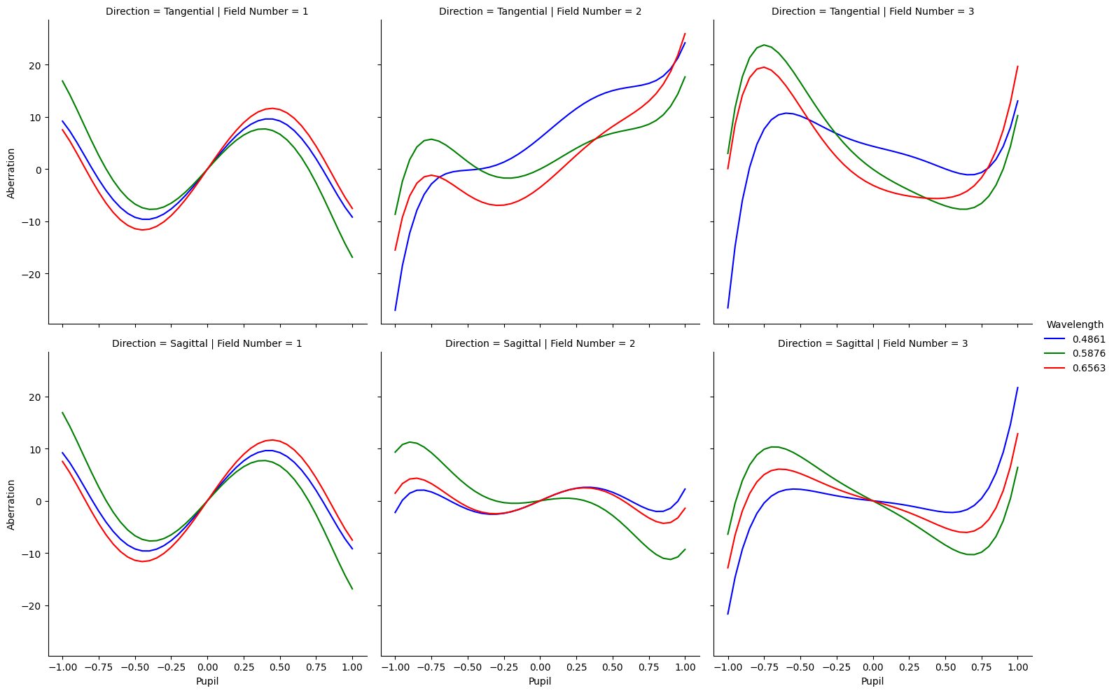
光线扇分析#
运行光线扇分析并绘制结果。
[6]:
ray_fan_result = zp.analyses.raysandspots.RayFan(number_of_rays=20, wavelength="All", field="All").run(oss)

sns.relplot(
    ray_fan_result.data.to_dataframe(),
    x="Pupil",
    y="Aberration",
    row="Direction",
    col="Field Number",
    hue="Wavelength",
    kind="line",
    palette=colors,
)
[6]:
<seaborn.axisgrid.FacetGrid at 0x2c076508c50>